Portfolio optimisation: the weights can amplify estimation error

An optimiser can solve its mathematical problem accurately and still produce an unstable portfolio. The problem may live in the estimated inputs: two almost identical assets, a noisy return difference and a risk model assigning very little variance to the spread between them.

We can see the mechanism with two assets and one weight. No market dataset is needed. The numbers below are deliberately specified teaching inputs, allowing us to separate the algebra from any claim about forecast accuracy.

Both assets have annual volatility 20%, correlation 0.99 and a fully invested portfolio. Asset B's expected annual return is fixed at 8.1%. We vary A's estimate by small amounts and watch the optimiser respond.

Write the one-dimensional objective

Put weight w in A and 1 − w in B. The mean–variance objective is expected return minus half of gamma times variance, with gamma = 4 under this particular annual decimal-return convention.

The covariance is 0.99 × 0.2 × 0.2 = 0.0396. Expanding the variance gives 0.04 − 0.0008w + 0.0008w². Its curvature in w is small because moving capital between almost identical assets changes the modelled portfolio risk only slightly.

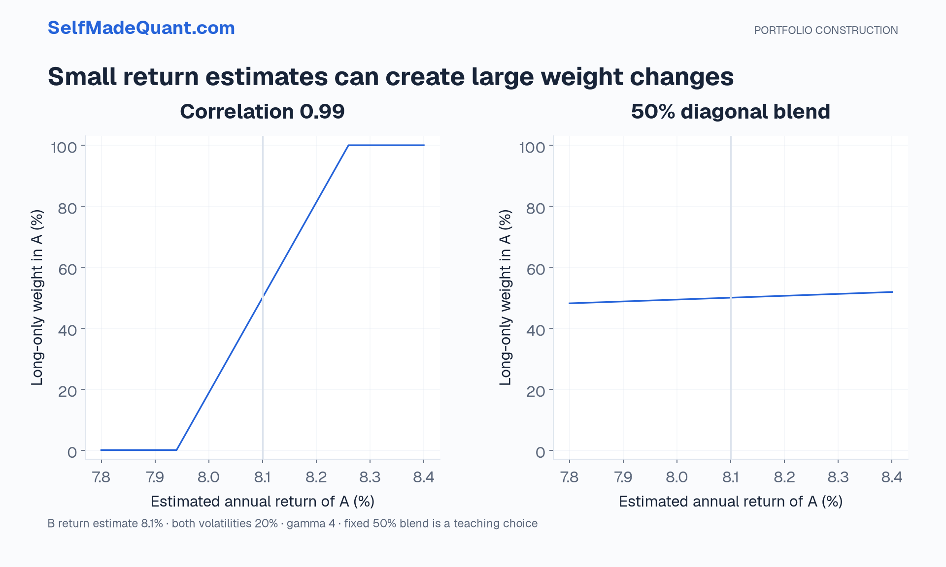
Setting the objective derivative to zero gives w = 0.5 + (muA − muB)/0.0032. With muA = 8.0%, w is 18.75%. With muA = 8.1%, it is 50%. With muA = 8.2%, it is 81.25%.

A ten-basis-point change in the expected-return estimate moves the weight by 31.25 percentage points. The arithmetic is correct. The economic question is whether the estimated return difference deserves that confidence.

A constraint changes the solution at the boundary

With a long-only constraint, w must lie between zero and one. In this concave two-asset problem, the constrained optimum is the unconstrained solution clipped to that interval. At sufficiently large estimated return differences, the solution becomes all A or all B.

That clipping rule is specific to this one-dimensional feasible interval. In a many-asset problem, clipping individual weights and renormalising does not generally solve the original constrained optimisation. Constraints interact through the budget and covariance matrix.

Similarly, a maximum position weight can prevent an extreme allocation without repairing the forecast that pushed towards it. A useful report describes both the binding constraint and the estimated input responsible for the pressure against it.

Shrinkage changes the risk estimate

Consider an illustrative covariance blend: half the original covariance matrix and half its diagonal. The variances stay at 0.04; the covariance falls from 0.0396 to 0.0198. The blend remains a valid positive-definite covariance matrix here.

The spread direction now carries more modelled risk. The same ten-basis-point expected-return change moves the unconstrained weight by about 0.62 percentage points instead of 31.25.

This is a controlled numerical demonstration. It does not establish that 50% shrinkage is optimal, or that zero correlation is the best target. A fixed blend is not automatically the Ledoit–Wolf estimator; that estimator includes a specific method for choosing shrinkage intensity.

Shrinking towards a structured target trades flexibility against estimation stability. Evaluate that choice with a stated estimation procedure and data window, rather than selecting the blend because it won the same backtest used to advertise the result.

Check the matrix and the horizon

Verify symmetry, positive semidefiniteness and asset ordering. Inspect whether near-zero eigenvalues correspond to duplicated assets or a genuinely well-measured hedging direction. A numerical inverse can make a weakly identified direction look precise.

In implementation, solve linear systems rather than explicitly forming an inverse when possible. That improves numerical practice, but it cannot remove uncertainty in the estimated covariance matrix. Numerical conditioning and statistical estimation are related problems, not interchangeable ones.

Expected returns and covariances must refer to compatible horizons and units. Changing a covariance's annualisation without changing the objective's expected returns or risk-aversion convention changes the optimisation problem.

Report sensitivity alongside weights

Show the base allocation and a small set of predeclared input perturbations. Which mean changes move the portfolio most? Which correlations make a concentration appear attractive? Which constraints bind? How much trade does each alternative require from current holdings?

A stable numerical solution is easier to review when the report also exposes the assumptions that keep it stable. The output should make the risk of input error visible, rather than letting a precise weight imply a precise forecast.

Until then, peace.