Transformations, Compositions, and Building New Functions

What this note is about

Pricing a barrier option, seasonally adjusting a commodity price, or applying an activation function in a neural network all involve taking a familiar function and modifying it — shifting its graph, scaling its values, or feeding one function's output into another. This note makes those operations precise. Three mechanisms are covered: graph transformations (shifting, stretching, reflecting), arithmetic combinations (sums, products, quotients), and the composition operator. Knowing how to read a composed function apart — identifying the outer function and the inner function — is the indispensable prerequisite for the chain rule.

Learning objectives. By the end of this note you should be able to:

apply the six canonical graph transformations to sketch $y = cf(x-a) + b$ from a known graph of $y = f(x)$ ;
determine the domains of sums, products, quotients, and compositions of two functions;
decompose a given function into outer and inner parts and name both;
identify when absolute-value wrapping reflects a function's graph.

Graph transformations

Given the graph of $y = f(x)$ , seven canonical transformations produce related graphs. Divide them into two groups.

Translations (shifts)

Proposition 1 (Vertical and horizontal shifts). Let

c > 0

Transformed function	Effect on graph
$y = f(x) + c$	shift up by $c$
$y = f(x) - c$	shift down by $c$
$y = f(x - c)$	shift right by $c$
$y = f(x + c)$	shift left by $c$

Intuition. To shift the graph right by

c

, you must replace

x

with

x - c

in the formula. That is, to achieve the same

y

-value, the new

x

must be

c

units further to the right. The sign is opposite to the direction of shift — this is the most common sign error in transformations.

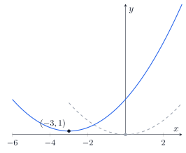
Example 1 (Shifted parabola). Given

y = x^2

, express

y = x^2 + 6x + 10

in terms of a shift.

Complete the square:

x^2 + 6x + 10 = (x + 3)^2 + 1

. This is

y = x^2

shifted 3 units left and 1 unit up. The vertex moves from

(0, 0)

(-3, 1)

Graph of y = x² (grey, vertex at origin) and its shift y = (x+3)² + 1 (blue, vertex at (−3,1)), showing the 3-left, 1-up translation

Stretches and reflections

Proposition 2 (Vertical and horizontal stretching/reflecting). Let

c > 1

Transformed function	Effect
$y = cf(x)$	stretch vertically by factor $c$
$y = (1/c)f(x)$	compress vertically by factor $c$
$y = f(cx)$	compress horizontally by factor $c$
$y = f(x/c)$	stretch horizontally by factor $c$
$y = -f(x)$	reflect about the $x$ -axis
$y = f(-x)$	reflect about the $y$ -axis

Financial interpretation. A log-return distribution

p(x)

can be rescaled to any volatility

\sigma

by the horizontal stretch

p(x/\sigma)/\sigma

— the standard-deviation rescaling that converts a unit-normal density to a

N(0, \sigma^2)

density. This is precisely the role of the

1/\sigma

Jacobian in a change-of-variables density computation.

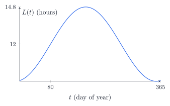
Example 2 (Daylight model). Philadelphia's daylight hours as a function of day-of-year

t

follow approximately

L(t) = 12 + 2.8 \sin\!\left(\tfrac{2\pi}{365}(t - 80)\right)

. Starting from

y = \sin t

: stretch vertically by 2.8, stretch horizontally by

365/(2\pi)

(period 365 days instead of

2\pi

), shift right by 80 days, then shift up by 12. Each transformation has a direct physical meaning: amplitude controls the day-length swing; the horizontal stretch controls the annual period; the right-shift places the minimum on December 21 (day

80

before the vernal equinox).

Graph of L(t) = 12 + 2.8 sin((2π/365)(t − 80)) over one year, oscillating between about 9.2 and 14.8 hours with the shifted, stretched sine shape

Absolute value as a reflection

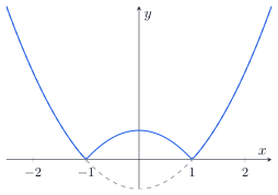
If $y = |f(x)|$ , the part of the graph of $f$ that lies below the $x$ -axis gets reflected above it. The part above stays put.

Example 3. To graph

y = |x^2 - 1|

: first draw

y = x^2 - 1

(parabola, vertex

(0, -1)

, zeros at

\pm 1

). The segment between

x = -1

and

x = 1

dips below the axis; reflect it up. The result is a "W" shape with vertex at

(0, 1)

and zeros at

\pm 1

Graph of y = x² − 1 (grey, dipping to −1 between the zeros) and y = |x² − 1| (blue), showing the below-axis segment reflected upward into a "W" shape

Arithmetic combinations

Given functions $f$ and $g$ with domains $A$ and $B$ :

Definition 1 (Arithmetic combinations). On the intersection

A \cap B

\begin{aligned} (f + g)(x) &= f(x) + g(x) \\ (f - g)(x) &= f(x) - g(x) \\ (fg)(x) &= f(x)\,g(x) \\ (f/g)(x) &= f(x)/g(x), \quad g(x) \neq 0 \end{aligned}

The domain of $f + g$ , $f - g$ , and $fg$ is $A \cap B$ . The domain of $f/g$ is $A \cap B$ with all points where $g = 0$ removed.

Example 4 (Domain of a combination). Let

f(x) = \sqrt{x}

(domain

[0, \infty)

) and

g(x) = \sqrt{2 - x}

(domain

(-\infty, 2]

). Then:

$(f + g)(x) = \sqrt{x} + \sqrt{2-x}$ , domain $[0, 2]$ .
$(f/g)(x) = \sqrt{x}/\sqrt{2-x}$ , domain $[0, 2)$ (exclude $x = 2$ where $g = 0$ ).

Composition

The most important way to build new functions is by feeding one into another.

Definition 2 (Composition). The composite of

f

after

g

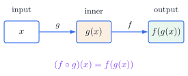
\boxed{(f \circ g)(x) = f(g(x))}

Domain of $f \circ g$ : all $x$ in the domain of $g$ such that $g(x)$ is in the domain of $f$ .

Symbol by symbol:

g

acts first (the inner function), producing an intermediate value

u = g(x)

; then

f

acts on that value (the outer function), producing the final output

f(u)

Composition flow diagram: input x passes through inner function g to produce g(x), then through outer function f to produce f(g(x)) = (f ∘ g)(x)

Example 5 (Identifying inner and outer). Let

h(x) = \sqrt{x^2 + 1}

Inner function: $g(x) = x^2 + 1$ . Outer function: $f(u) = \sqrt{u}$ . Then $h = f \circ g$ since $f(g(x)) = \sqrt{x^2 + 1}$ . Domain: all $x$ (since $x^2 + 1 \geq 1 > 0$ for all real $x$ ).

Remark 1 (Order matters). Composition is not commutative. In general

f \circ g \neq g \circ f

. For

f(x) = \sqrt{x}

and

g(x) = x + 1

$(f \circ g)(x) = \sqrt{x + 1}$ , domain $[-1, \infty)$ .
$(g \circ f)(x) = \sqrt{x} + 1$ , domain $[0, \infty)$ .

Different functions with different domains. Never write $f \circ g = g \circ f$ without checking.

Example 6 (Decomposing a finance function). The Black-Scholes

d_1

formula contains the term

\ln(S/K)/(sigma\sqrt{T})

. Identify the compositional structure.

Let $h = \ln(S/K)$ . This is $h = \ln \circ (\cdot/K)$ : first divide by $K$ (inner), then take the natural log (outer). The whole fraction $d_1 = [\ln(S/K) + (r + \sigma^2/2)T]/(\sigma\sqrt{T})$ is a linear function of $\ln(S/K)$ — a composition of the logarithm with the ratio $S/K$ and then a linear scaling. Recognising this structure is what allows you to differentiate $d_1$ with respect to $S$ , $\sigma$ , or $T$ via the chain rule.

Remark 2 (Decomposition is not unique). Most composed functions can be decomposed in more than one way. For

h(x) = (x^2 + 1)^{10}

, valid choices include: outer

f(u) = u^{10}

, inner

g(x) = x^2 + 1

; or outer

f(u) = (u+1)^{10}

, inner

g(x) = x^2

. The convention for the chain rule is to use the most natural outer/inner split — usually the one that reveals the most structure in the expression.

Even and odd functions

Definition 3. A function

f

is even if

f(-x) = f(x)

for all

x

in its domain (graph symmetric about the

y

-axis). It is odd if

f(-x) = -f(x)

for all

x

(graph symmetric about the origin).

Most functions are neither even nor odd. Polynomials with only even powers are even; polynomials with only odd powers are odd.

Financial connection. Payoff distributions for straddles are symmetric about the current spot — an even payoff around

K

. Skewed payoffs (risk reversals, digital puts vs calls) are explicitly odd-symmetric perturbations of a symmetric base.

Where this goes next

Exponential Functions, Logarithms, and the Number e: the most important composition target in finance — $e^x$ composed with a linear function of time gives continuous compounding.
The Chain Rule: the differentiation rule for compositions; every application in finance — Greeks of composed payoffs, sensitivity of log-prices — reduces to this.
Implicit Differentiation and Logarithmic Derivatives: differentiates compositions where the output is not explicitly isolated.

Exercises

Exercise 1. Starting from the graph of

y = \sqrt{x}

, describe in order the transformations needed to obtain

y = -2\sqrt{x - 3} + 1

. State the domain and range of the result.

Solution. Apply in sequence to

y = \sqrt{x}

Replace $x$ with $x - 3$ : shift right 3 → $y = \sqrt{x - 3}$ , domain $[3, \infty)$ .
Multiply by 2: stretch vertically by 2 → $y = 2\sqrt{x - 3}$ , range $[0, \infty)$ .
Multiply by $-1$ : reflect about the $x$ -axis → $y = -2\sqrt{x - 3}$ , range $(-\infty, 0]$ .
Add 1: shift up 1 → $y = -2\sqrt{x - 3} + 1$ , range $(-\infty, 1]$ .

Domain: $[3, \infty)$ ; range: $(-\infty, 1]$ . $\blacksquare$

Exercise 2. Find the domain of

h(x) = \dfrac{\sqrt{x-1}}{x^2 - 9}

Solution. Write

h = f/g

where

f(x) = \sqrt{x - 1}

(domain

[1, \infty)

) and

g(x) = x^2 - 9

(domain

\mathbb{R}

). The domain of

h

(A \cap B) \setminus \{g = 0\}

$g(x) = 0 \Leftrightarrow x = \pm 3$ . On $[1, \infty)$ , the point $x = -3$ is already excluded; $x = 3$ must be removed.

Domain: $[1, 3) \cup (3, \infty)$ . $\blacksquare$

Exercise 3. Let

f(x) = \dfrac{1}{x}

and

g(x) = x^2 - 1

(a) Find $f \circ g$ and its domain.
(b) Find $g \circ f$ and its domain.
(c) Show $f \circ g \neq g \circ f$ .

Solution. (a)

(f \circ g)(x) = f(g(x)) = 1/(x^2 - 1)

. Domain:

\mathbb{R} \setminus \{\pm 1\}

(exclude where

g = 0

, i.e.

x = \pm 1

(b) $(g \circ f)(x) = g(f(x)) = (1/x)^2 - 1 = 1/x^2 - 1$ . Domain: $\mathbb{R} \setminus \{0\}$ (exclude $x = 0$ where $f$ is undefined).

(c) Take $x = 2$ : $(f \circ g)(2) = 1/(4-1) = 1/3$ ; $(g \circ f)(2) = 1/4 - 1 = -3/4$ . Different values, confirming $f \circ g \neq g \circ f$ . $\blacksquare$

Exercise 4 (Decomposition — finance application). A risk system computes a position's dollar Greeks by the formula

\text{Dollar Delta} = \Delta \cdot S

where $\Delta = N(d_1)$ (the option delta, a function of the log-moneyness $m = \ln(S/K)$ ) and $S$ is the current spot price. Express the dollar delta as a composed function and identify the outer and inner functions when the independent variable is $S$ .

Solution. Write the dollar delta as

H(S) = N(d_1(S)) \cdot S

. This is a product of two functions, not a composition; but each factor involves composition:

$d_1(S) = [\ln(S/K) + (r + \sigma^2/2)T]/(\sigma\sqrt{T})$ : outer is the affine map $u \mapsto (u + c_1)/c_2$ (where $c_1, c_2$ are constants), inner is $\ln(\cdot/K)$ — itself the logarithm composed with the scaling $S \mapsto S/K$ .
$N(d_1(S))$ : outer is the standard normal CDF $N$ , inner is $d_1(S)$ .

Dollar delta

= N(d_1(S)) \cdot S

is the product of the two composed functions. To differentiate with respect to

S

later, the chain rule is applied to each factor. Identifying the composition structure here is precisely what lets us read off the option gamma as

\partial \Delta/\partial S = n(d_1) / (S\sigma\sqrt{T})

, where

n = N'

is the standard normal density.

\blacksquare

This is a sample from the full curriculum. Members get every lesson, exercise solution and project.

See membership options

Another free sample

Options pricing · Binomial treesThe Binomial ModelBuild a recombining price tree and understand the risk-neutral probabilities behind option valuation.