The Binomial Model

What this note is about

The binomial tree is the computational engine for every contract that breaks the Black–Scholes closed form: American early exercise and path-dependent barriers both reduce to the same backward-induction pass with a one-line modification. This note sets up the model — the assumptions (Bi1)–(Bi3), why the tree recombines, and how the three parameters

u

d

p

are pinned down by forcing the discrete model to imitate risk-neutral GBM over each step. Two equations match mean and variance; the third is a free design choice whose classic value

\gamma = 1

(Cox–Ross–Rubinstein) gives a symmetric tree ideal for barriers. The full algebra lives in the CRR-parameter derivation.

Learning objectives. By the end of this note you should be able to:

state the binomial assumptions (Bi1)–(Bi3) and explain why the tree recombines;
derive the mean-matching equation and the risk-neutral probability $q$ ;
derive the variance-matching equation and explain the role of the third equation $ud = \gamma$ ;
quote the exact CRR solution and its approximation $u \approx e^{\sigma\sqrt{\Delta t}}$ , and interpret it;
compute $u, d, p$ numerically for given $r, \sigma, \Delta t$ .

One-step binomial model and replication

Refresher from market model and risk-neutral valuation: over one period the stock moves

S_0 \to S_0 u

S_0 \to S_0 d

with

0 < d < e^{r\Delta t} < u

. Replicating the option with

\Delta

shares and cash forces

\Delta = \frac{V^u - V^d}{S_0 (u - d)}, \qquad V_0 = e^{-r\Delta t}\left[ q V^u + (1-q) V^d \right], \qquad q = \frac{e^{r\Delta t} - d}{u - d}.

Here

V^u, V^d

are the option's known values in the two successor states, and

q

is the risk-neutral probability: it is a genuine probability (

0 < q < 1

) exactly when

d < e^{r\Delta t} < u

, which is forced by no-arbitrage . Under

q

\mathbb{E}^{\mathbb{Q}}[S_{\Delta t}] = S_0 e^{r\Delta t}

. Real-world probabilities never enter.

Financial interpretation. The hedge ratio

\Delta

is the discrete ancestor of

\partial V/\partial S

. Pricing by replication and pricing by discounted risk-neutral expectation give the same number because the price is the cost of the hedge.

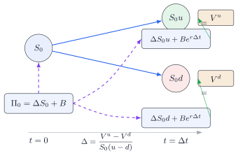
One-step binomial tree: stock moves to S_0 u or S_0 d; a portfolio of \Delta shares plus B in the bond replicates the option payoffs V^u and V^d at t=\Delta t, with \Delta=(V^u-V^d)/(S_0(u-d))

Remark 1.1 (completeness). With two unknowns in the hedge portfolio (shares and cash) and two future states, replication has a unique solution for any payoff — the one-step market is complete. This is the entire reason the binomial model prices uniquely; with three or more states per step a single stock and bond could no longer replicate everything .

The multi-step tree

Divide $[0, T]$ into $M$ steps, $\Delta t = T/M$ , $t_i = i \Delta t$ .

Assumptions 1.2 (Bi1)–(Bi3).

(Bi1) over each $\Delta t$ , $S \to Su$ or $S \to Sd$ , with $0 < d < u$ and the same $u, d$ at every node;
(Bi2) $\mathbb{P}(\text{up}) = p$ , the same at every node;
(Bi3) expectation and variance of the discrete model match those of continuous risk-neutral GBM.

(Bi1)+(Bi2) make the tree homogeneous; (Bi3) is the calibration requirement that makes the tree a discretisation of our model rather than an arbitrary lattice.

Proposition 1.3 (node values and recombination). The node reached by

n

up-moves out of

m

steps has value

S_n^m = u^n d^{\,m-n} S_0, \qquad n = 0, 1, \dots, m .

Because

S u d = S d u

, the order of moves is irrelevant — the tree recombines: after

m

steps there are only

m+1

distinct values, not

2^m

, and the total node count grows quadratically in

M

Three-step CRR binomial tree (S_0=100, u\approx1.162, d\approx0.861): up-then-down and down-then-up paths meet at the same node (100), so M=3 yields four terminal prices, not eight

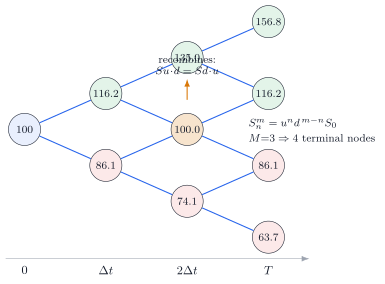
Why recombination matters computationally:

2^{100} \approx 10^{30}

paths vs

\sim 5000

nodes for

M = 100

. Recombination is the difference between exponential and polynomial cost. (It breaks when discrete dividends shift nodes off the lattice — see backward induction and the binomial algorithm.)

At expiry there are $M+1$ terminal prices $S_{j,M} = S_0 u^j d^{M-j}$ , spanning $[S_0 d^M,\ S_0 u^M]$ .

Deriving $u$ , $d$ , $p$ — matching the continuous model

Three unknowns need three equations. The first two implement (Bi3); the third is ours to choose.

Equation 1 — match the mean. Discrete one-step mean:

\mathbb{E}[S_{i+1}] = p S_i u + (1-p) S_i d

. Continuous risk-neutral GBM:

\mathbb{E}[S_{i+1}] = S_i e^{r\Delta t}

. Equating and dividing by

S_i

p u + (1-p) d = e^{r\Delta t} \quad\Longrightarrow\quad p = \frac{e^{r\Delta t} - d}{u - d}.

Note this is the same

q

as in section 1: matching the risk-neutral mean and pricing by replication produce one number.

Equation 2 — match the variance. Continuous risk-neutral GBM satisfies

\mathbb{E}[S_{i+1}^2] = S_i^2 e^{(2r + \sigma^2)\Delta t}

, so per unit

S_i^2

p u^2 + (1-p) d^2 = e^{(2r + \sigma^2)\Delta t} .

This is where $\sigma$ enters the tree — the spread between $u$ and $d$ must reproduce the model's variance.

Equation 3 — a free design choice. Impose

u\, d = \gamma

for a chosen constant

\gamma

. The classic choice is

\gamma = 1

(Cox–Ross–Rubinstein): symmetric up/down moves, so the tree's central line grows vertically.

Theorem 1.4 (CRR solution). With

\gamma = 1

and

\beta := \tfrac12 \left( e^{-r\Delta t} + e^{(r+\sigma^2)\Delta t} \right)

\boxed{\;u = \beta + \sqrt{\beta^2 - 1}, \qquad d = 1/u = \beta - \sqrt{\beta^2 - 1}, \qquad p = \frac{e^{r\Delta t} - d}{u - d}\;}

Up to higher-order terms in

\Delta t

this gives the familiar CRR parameters

u \approx e^{\sigma\sqrt{\Delta t}} \approx 1 + \sigma\sqrt{\Delta t}, \qquad d \approx e^{-\sigma\sqrt{\Delta t}} .

Full step-by-step algebra: the CRR-parameter derivation.

Remark 1.5 (reading the solution). The tree's vertical extension per step is

\pm\sigma\sqrt{\Delta t}

in log-space — one standard deviation of the continuous model's log-return. The

\sqrt{\Delta t}

is the diffusive scaling from stochastic processes, Brownian motion and Itô's lemma: noise grows like the square root of time, and so must the lattice.

Example 1.6 (numerical calibration). Take

r = 0.05

\sigma = 0.3

T = 1

M = 4

, so

\Delta t = 0.25

. CRR approximation:

u = e^{0.3\sqrt{0.25}} = e^{0.15} \approx 1.1618, \qquad d = 1/u \approx 0.8607,

p = \frac{e^{0.05 \times 0.25} - 0.8607}{1.1618 - 0.8607} \approx 0.5044 .

Sanity checks: $d < e^{r\Delta t} \approx 1.0126 < u$ ✓; $p \in (0,1)$ ✓.

Summary table — the three ingredients:

Requirement	Equation	Consequence
no-arbitrage / martingale mean	$pu + (1-p)d = e^{r\Delta t}$	$p = \frac{e^{r\Delta t} - d}{u-d}$ , valid iff $d < e^{r\Delta t} < u$
volatility matching	$pu^2 + (1-p)d^2 = e^{(2r+\sigma^2)\Delta t}$	spread $u, d \sim e^{\pm\sigma\sqrt{\Delta t}}$
normalisation $ud = \gamma$	free choice	$\gamma = 1$ : symmetric tree (good for barriers); $\gamma = \exp\big(\frac{2}{M}\log\frac{K}{S_0}\big)$ : tilted tree (good convergence)

Exercises

Exercise 1.1. Verify that with the exact CRR solution (Theorem 1.4), Equations 1 and 2 hold identically.

Solution. Since

u, d = \beta \pm \sqrt{\beta^2 - 1}

, we have

ud = 1

and

u + d = 2\beta = e^{-r\Delta t} + e^{(r+\sigma^2)\Delta t}

. Equation 1 holds by construction of

p

. For Equation 2, using

p(u-d) = e^{r\Delta t} - d

pu^2 + (1-p)d^2 = d^2 + (e^{r\Delta t} - d)(u+d) = e^{r\Delta t}(u+d) - ud = e^{(2r+\sigma^2)\Delta t}. \checkmark \qquad \blacksquare

**Exercise 1.2 . Expand

\beta

and

u = \beta + \sqrt{\beta^2-1}

in powers of

\sqrt{\Delta t}

to show

u = e^{\sigma\sqrt{\Delta t}}\big(1 + O(\Delta t^{3/2})\big)

Solution. With

\varepsilon = \Delta t

\beta = 1 + \tfrac12\sigma^2\varepsilon + O(\varepsilon^2)

, so

\sqrt{\beta^2 - 1} = \sigma\sqrt{\varepsilon} + O(\varepsilon^{3/2})

and

u = 1 + \sigma\sqrt{\varepsilon} + \tfrac12\sigma^2\varepsilon + O(\varepsilon^{3/2}) = e^{\sigma\sqrt{\Delta t}} + O(\Delta t^{3/2})

\blacksquare

Exercise 1.3. For

r = 0.05

\sigma = 0.3

M = 4

S_0 = 100

, write out all five terminal stock prices and verify the tree spans

S_0 e^{\pm 2\sigma\sqrt{T}}

Solution. Terminal nodes:

S_{j,4} = 100\,e^{0.15(2j-4)}

giving

\{54.88, 74.08, 100.00, 134.99, 182.21\}

. Span:

2\sigma\sqrt{T} = 0.6

, matching

e^{\pm 0.6}

\blacksquare

Exercise 1.4. A colleague proposes

u = 1.01

d = 0.99

\Delta t = 0.25

r = 5\%

. Show that

q \notin (0,1)

and construct the explicit arbitrage.

Solution.

e^{r\Delta t} = 1.012578 > u = 1.01

, so

q = 1.129 \notin (0,1)

. Short the stock, deposit proceeds: profit

S_0(1.012578 - 1.01) > 0

in the up state and

S_0(1.012578 - 0.99) > 0

in the down state — riskless profit above the bank rate.

\blacksquare

**Exercise 1.5 . Explain in one paragraph why Shreve's multi-period model uses the same

u, d, q

at every node rather than calibrating locally to a term structure of volatility.

Solution. Homogeneous

(u,d,q)

make the tree recombining and keep node count

O(M^2)

. Local calibration would break recombination (each node carries its own geometry), exploding memory to

O(2^M)

unless a state-space collapse is engineered. For equity options with flat

\sigma

the homogeneous tree is the standard; term-structure effects require implied-vol interpolation or a trinomial tree with time-dependent parameters .

\blacksquare

This is a sample from the full curriculum. Members get every lesson, exercise solution and project.

See membership options

Another free sample

Mathematics · Calculus ITransformations, Compositions, and Building New FunctionsShift, scale, and compose functions — from familiar graphs to the building blocks of financial models.

What this note is about

One-step binomial model and replication

The multi-step tree

Deriving uuu, ddd, ppp — matching the continuous model

Exercises

Another free sample

Deriving $u$ , $d$ , $p$ — matching the continuous model